Numba vs Numpy: some sums
Numba is open-source optimizing compiler for Python. It seems work like magic: just add a simple decorator to your pure-python function, and it immediately becomes 200 times faster – at least, so clames the Wikipedia article about Numba. Even this is hard to believe, but Wikipedia goes further and claims that a vary naive implementation of a sum of a numpy array is 30% faster then numpy.sum. Somehow, I would expect that numpy.sum is as optimized as it can be, so this clame sounds even more ambitious. Let’s check this with some benchmarks!
System setup 
As usual, I’m working on my Lenovo T440p laptop running AltLinux. It has mobile Haswell processor with 2 cores and 4 hardware threads. To make benchmarks more reproducible, I’ve disabled TurboBoost and locked scaling to almost 2 GHz (~1995).
%%sh
uname -a
Linux imelnikov.localdomain 4.14.24-un-def-alt0.M80P.1 #1 SMP PREEMPT Tue Mar 6 15:00:33 UTC 2018 x86_64 GNU/Linux
%%sh
cat /proc/cpuinfo | egrep '^model name|Hz'
model name	: Intel(R) Core(TM) i5-4300M CPU @ 2.60GHz
cpu MHz		: 1995.544
model name	: Intel(R) Core(TM) i5-4300M CPU @ 2.60GHz
cpu MHz		: 1995.545
model name	: Intel(R) Core(TM) i5-4300M CPU @ 2.60GHz
cpu MHz		: 1995.545
model name	: Intel(R) Core(TM) i5-4300M CPU @ 2.60GHz
cpu MHz		: 1995.543
Let’s import some modules and check the versions:
import sys
import numba
import numpy as np
import matplotlib.pyplot as plt
plt.style.use('ggplot')
print("python version:", ''.join(sys.version.splitlines()))
print("numpy version:", np.__version__)
print("numba version:", numba.__version__)
python version: 3.6.4 |Anaconda custom (64-bit)| (default, Jan 16 2018, 18:10:19) [GCC 7.2.0]
numpy version: 1.14.0
numba version: 0.36.2
np.random.seed(42)
System under test 
Here is the code from Wikipedia:
def sum1d(my_double_array):
    total = 0.0
    for i in range(my_double_array.shape[0]):
        total += my_double_array[i]
    return total
Numba’s jit is intended to be used as decorator, but we’re going to call it explicitly to make sure we run the same code with and without jit:
sum1d_jit = numba.jit(nopython=True)(sum1d)
sum1d_jit
CPUDispatcher(<function sum1d at 0x7fb4eee77158>)
We’ll also check if parallelization will make any difference for us:
sum1d_par = numba.jit(nopython=True, parallel=True)(sum1d)
Let’s run a quick test to make sure we’ve done everything correctly, and to force numba to compile float64 version of our sum1d:
sample_data = np.random.randn(42)
sum1d(sample_data), sum1d_jit(sample_data), sum1d_par(sample_data), np.sum(sample_data)
(-7.835638675532193,
 -7.835638675532193,
 -7.835638675532193,
 -7.835638675532195)
It’s interesting: naive python version and jitted version return the same number exactly, but numpy.sum apparently calculates things in a bit differntly.
Measurements 
We’ll make a few runs for various array sizes:
measures = 13
sizes = 4 ** np.arange(measures)
We’ll save the average runtime here:
res_numpy = np.zeros(measures)
res_python = np.zeros(measures)
res_numba = np.zeros(measures)
res_numba_par = np.zeros(measures)
It’s time to measures all the things! This will take a few minutes:
%%time
for idx, size in enumerate(sizes):
    print("size =", size)
    data = np.random.randn(size).astype('f8')
    res = %timeit -o np.sum(data)
    res_numpy[idx] = res.average
    res = %timeit -o sum1d(data)
    res_python[idx] = res.average
    res = %timeit -o sum1d_jit(data)
    res_numba[idx] = res.average
    res = %timeit -o sum1d_par(data)
    res_numba_par[idx] = res.average
del data
size = 1
5.53 µs ± 298 ns per loop (mean ± std. dev. of 7 runs, 100000 loops each)
1.04 µs ± 93.7 ns per loop (mean ± std. dev. of 7 runs, 1000000 loops each)
448 ns ± 8.96 ns per loop (mean ± std. dev. of 7 runs, 1000000 loops each)
469 ns ± 19.5 ns per loop (mean ± std. dev. of 7 runs, 1000000 loops each)
size = 4
4.07 µs ± 182 ns per loop (mean ± std. dev. of 7 runs, 100000 loops each)
1.6 µs ± 26.5 ns per loop (mean ± std. dev. of 7 runs, 1000000 loops each)
473 ns ± 6.14 ns per loop (mean ± std. dev. of 7 runs, 1000000 loops each)
453 ns ± 6.65 ns per loop (mean ± std. dev. of 7 runs, 1000000 loops each)
size = 16
4.17 µs ± 205 ns per loop (mean ± std. dev. of 7 runs, 100000 loops each)
4.35 µs ± 172 ns per loop (mean ± std. dev. of 7 runs, 100000 loops each)
526 ns ± 77.8 ns per loop (mean ± std. dev. of 7 runs, 1000000 loops each)
585 ns ± 26 ns per loop (mean ± std. dev. of 7 runs, 1000000 loops each)
size = 64
4.54 µs ± 418 ns per loop (mean ± std. dev. of 7 runs, 100000 loops each)
16.6 µs ± 2.29 µs per loop (mean ± std. dev. of 7 runs, 100000 loops each)
678 ns ± 46.8 ns per loop (mean ± std. dev. of 7 runs, 1000000 loops each)
676 ns ± 22.4 ns per loop (mean ± std. dev. of 7 runs, 1000000 loops each)
size = 256
5.89 µs ± 401 ns per loop (mean ± std. dev. of 7 runs, 100000 loops each)
75.3 µs ± 1.61 µs per loop (mean ± std. dev. of 7 runs, 10000 loops each)
1.02 µs ± 35.7 ns per loop (mean ± std. dev. of 7 runs, 1000000 loops each)
958 ns ± 14.4 ns per loop (mean ± std. dev. of 7 runs, 1000000 loops each)
size = 1024
6.33 µs ± 228 ns per loop (mean ± std. dev. of 7 runs, 100000 loops each)
319 µs ± 32.8 µs per loop (mean ± std. dev. of 7 runs, 1000 loops each)
2.28 µs ± 169 ns per loop (mean ± std. dev. of 7 runs, 100000 loops each)
2.21 µs ± 118 ns per loop (mean ± std. dev. of 7 runs, 100000 loops each)
size = 4096
8.31 µs ± 158 ns per loop (mean ± std. dev. of 7 runs, 100000 loops each)
1.2 ms ± 49.9 µs per loop (mean ± std. dev. of 7 runs, 1000 loops each)
7.06 µs ± 59.2 ns per loop (mean ± std. dev. of 7 runs, 100000 loops each)
7.02 µs ± 23.4 ns per loop (mean ± std. dev. of 7 runs, 100000 loops each)
size = 16384
18.2 µs ± 323 ns per loop (mean ± std. dev. of 7 runs, 100000 loops each)
4.7 ms ± 149 µs per loop (mean ± std. dev. of 7 runs, 100 loops each)
26.7 µs ± 363 ns per loop (mean ± std. dev. of 7 runs, 10000 loops each)
26.5 µs ± 136 ns per loop (mean ± std. dev. of 7 runs, 10000 loops each)
size = 65536
52.9 µs ± 2.09 µs per loop (mean ± std. dev. of 7 runs, 10000 loops each)
19.7 ms ± 670 µs per loop (mean ± std. dev. of 7 runs, 100 loops each)
102 µs ± 950 ns per loop (mean ± std. dev. of 7 runs, 10000 loops each)
101 µs ± 144 ns per loop (mean ± std. dev. of 7 runs, 10000 loops each)
size = 262144
176 µs ± 3.17 µs per loop (mean ± std. dev. of 7 runs, 10000 loops each)
77.9 ms ± 6.35 ms per loop (mean ± std. dev. of 7 runs, 10 loops each)
440 µs ± 4.42 µs per loop (mean ± std. dev. of 7 runs, 1000 loops each)
457 µs ± 15.9 µs per loop (mean ± std. dev. of 7 runs, 1000 loops each)
size = 1048576
948 µs ± 36.6 µs per loop (mean ± std. dev. of 7 runs, 1000 loops each)
320 ms ± 18.3 ms per loop (mean ± std. dev. of 7 runs, 1 loop each)
1.89 ms ± 52.7 µs per loop (mean ± std. dev. of 7 runs, 1000 loops each)
1.86 ms ± 64.7 µs per loop (mean ± std. dev. of 7 runs, 1000 loops each)
size = 4194304
3.51 ms ± 67.8 µs per loop (mean ± std. dev. of 7 runs, 100 loops each)
1.22 s ± 27.5 ms per loop (mean ± std. dev. of 7 runs, 1 loop each)
7.31 ms ± 74.7 µs per loop (mean ± std. dev. of 7 runs, 100 loops each)
7.32 ms ± 77.5 µs per loop (mean ± std. dev. of 7 runs, 100 loops each)
size = 16777216
14.8 ms ± 583 µs per loop (mean ± std. dev. of 7 runs, 100 loops each)
4.87 s ± 116 ms per loop (mean ± std. dev. of 7 runs, 1 loop each)
29.2 ms ± 88.9 µs per loop (mean ± std. dev. of 7 runs, 10 loops each)
29.7 ms ± 349 µs per loop (mean ± std. dev. of 7 runs, 10 loops each)
CPU times: user 6min 4s, sys: 267 ms, total: 6min 5s
Wall time: 6min 5s
Looking at the data 
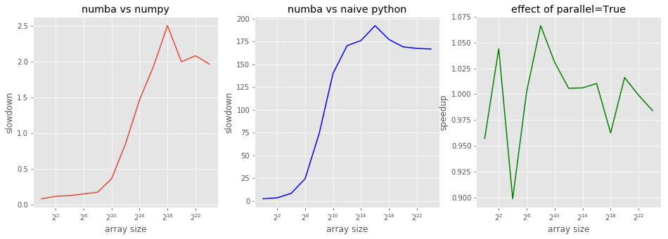
First, let’s look at various speedups and slowdowns:
numba_vs_naive = res_python / res_numba
numba_vs_naive.max()
192.3750032906321
Well, it’s not 200 times as Wikipedia claimed, but it’s pretty much close to it.
numba_vs_numpy = res_numba / res_numpy
numba_vs_numpy.min(), numba_vs_numpy.max()
(0.08103373848130296, 2.505059846262734)
Numba can be 2.5 times slower then numpy, but it can also be faster. Let’s look at the graphs below.
numba_vs_par = res_numba / res_numba_par
numba_vs_par.min(), numba_vs_par.max()
(0.8986877079731856, 1.0664777926145088)
Aparently, numba cannot parallelize our function – it’s too naive for that. Let’s look how speedups/slowdowns change with the array size:
fig, (ax1, ax2, ax3) = plt.subplots(1,3)

fig.set_size_inches(16, 5)

ax1.set_title('numba vs numpy')
ax1.set_xlabel('array size')
ax1.set_ylabel('slowdown')
ax1.semilogx(sizes, numba_vs_numpy, basex=2);


ax2.set_title('numba vs naive python')
ax2.set_xlabel('array size')
ax2.set_ylabel('slowdown')
ax2.semilogx(sizes, numba_vs_naive, basex=2, color='b');

ax3.set_title('effect of parallel=True')
ax3.set_xlabel('array size')
ax3.set_ylabel('speedup')
ax3.semilogx(sizes, numba_vs_par, basex=2, color='g');
plt.figure().set_size_inches(12, 10)
plt.loglog(sizes, res_numba, label='numba', basex=2)
plt.loglog(sizes, res_numba_par, label='numba parallel', basex=2)
plt.loglog(sizes, res_numpy, label='numpy', basex=2)
plt.loglog(sizes, res_python, label='naive python', basex=2)
plt.xlabel("array size")
plt.ylabel("runtime, seconds");
plt.legend();
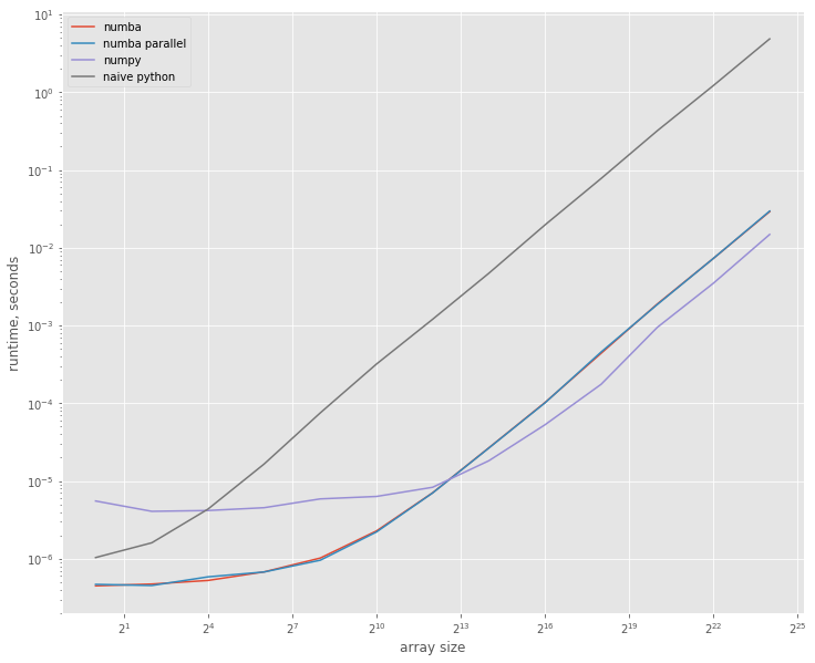
The jitted version is more then 5 times faster on smaller arrays, but for larger arrays numpy becomes ~2.5 times faster then numba; they show similar performance when array sizes are about 4000.
Conclusions 
I consider both clames of the Wikipedia article confirmed: numba brings tremendous speedup to naive python code at the const of just one decorator (and one huge additional dependency – the numba itself ^_-); for arrays of quite reasonable size numba can be much faster then numpy – e.g. for size 1024 it ~2 times faster!
This allows me to conclude that numba is awesome. Let’s see how it will behave on more real-life projects of mine.
You can download the full notebook here.